How the Histogram Works¶

When the Histogram receives an updated image from one of the monitors, each of these pixels consists of a Red, Green, and Blue component. Each of these values lies within a range of 0 and 255, which are the numbers you can represent with one Byte. 0 means that the component is not shining at all (i.e. it is black), 255 means that it is shining as bright as possible.

The histogram is merely statistics: it shows how often a component of a certain brightness occurs. So what the histogram then does is actually quite simple:

Take the first pixel
Look at the Red value (= x) of the pixel. Increase the height of the bar at position x of the histogram by 1. Example: If the red value is 0, increase the height of the bar at position 0 (that is at the very left) of the histogram by 1. If it is 42, increase bar 42 by 1. And so on.
Repeat the previous step with Green and Blue.
Look at R, G, and B together and calculate the Luma value. Luma is the perceived luminance of this pixel. See further below how it is calculated.
Repeat these steps for all other pixels on the image.

What the Histogram Shows¶

The Histogram only shows the distribution of the luminance of the selected components - nothing more, nothing less. Also when looking at the RGB channels separately instead of at the calculated Luma component only, you cannot really guess the colors in the image. Take a look at these two images:

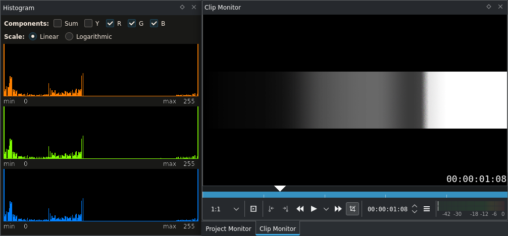
Histogram for a simple greyscale gradient image¶

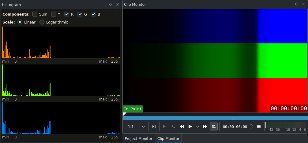
Histogram for a simple color gradient image¶

Exactly the same Histogram. Totally different colors. (What you can do is guessing the color tone; see below.) But what is the histogram good for now?

To answer this question, it is best to refer you to this article from Cambridge in Colour: Understanding Camera Histograms: Tones and Contrast and the second part Camera Histograms: Luminosity & Color. Although written for digital photo cameras, exactly the same applies for digital video cameras. Both articles are easy to read and understand and may also be of interest for experienced users.

Example 1: Candlelight¶

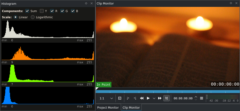
Histogram example with a candlelight image¶

Two special things about this histogram.

Most pixels are dark, according to the Luma component (white). Though there is no total black: Notice that the Luma component shows «min: 8». Nevertheless, the blue component does reach 0. This means that the darkest pixels are still slightly orange and didn't lose all color information yet.
There is quite some clipping. A lot of R values are sticking at the very right, at 255. Having a peak at 255 usually means that we lost information because some regions were too bright for the camera sensor with the current sensitivity settings. This could have been solved by lowering the sensitivity, but then the book and nearly everything else would be black. In this case the candles cause the clipping. (Not too bad here, because the lost detail isn't important for the image.)

The RGB components also show very well that the shadows are not neutral grey but orange, otherwise the color heaps on the left would, as in the gradient histogram above, have their center at the same position. There isn't a lot to correct here, what could be done is raising the shadows with a Courbes effect, but this is a matter of taste and the intended mood for the final movie.

Histogram before and after applying some color correcting with the Courbes effect¶

Example 2: Underexposed ABC¶

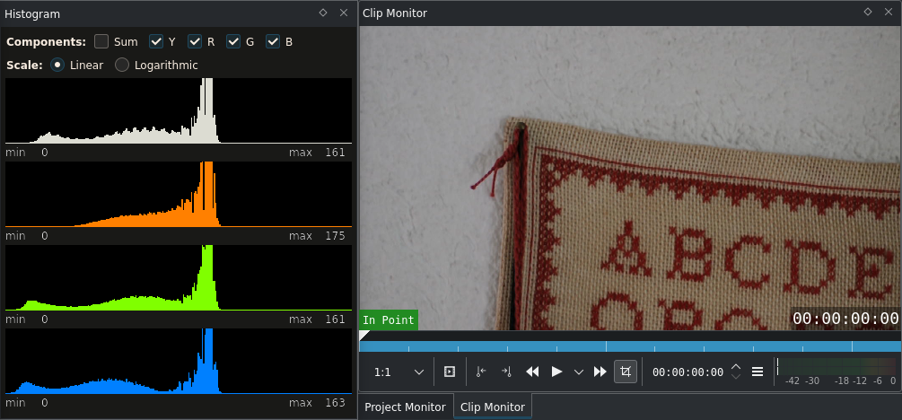
Histogram example 2 with an underexposed image¶

We immediately notice two things:

The RGB peaks are at the same position, near the middle. The white wall is the brightest part, so these peaks are from the white wall. As they are not shifted, the white balance should be okay (the image confirms that). Note that the Histogram is not very accurate for white balance. Later we will introduce a much more accurate scope.
The image is too dark. The brightest component, red, only reaches a value of 170. The white wall is actually grey.

Monitoring correct exposure is the histogram's strength! The exposure can be corrected with Courbes as well, but this time we will use the Niveaux effect.

Histogram before and after applying the Niveaux effect to correct exposure¶

We have lowered the input white level of the luma channel until one of the RGB components reached 255. Lowering the input white level further would cause clipping on the wall and loss of image information. (Which may be desired in certain circumstances!)

This process is called Stretching of the tonal range.

Histogram Options¶

The Histogram can be adjusted as follows:

Components - They can be enabled individually. For example, you might only want to see the Luma component, or you want to hide the Sum display.
- Y or Luma is the best known histogram. Every digital camera shows it, digiKam, GIMP, etc. know it. See below how it is calculated.
- Sum is basically a quick overview over the individual RGB channels. If it shows e.g. 5 as the minimum value, you know that none of the RGB components goes lower than 5.
- R / G / B show the histogram for the individual channels.
Unscaled (Context menu) - Does not scale the width of the histogram (unless the widget size is smaller). Just a goodie if you want to have it 256px wide.

Luma mode (Context menu) - This option defines how the Luma value of a pixel is calculated. Two options are available:
- Rec. 601 uses the formula Y' = 0.299 R' + 0.587 G' + 0.114 B'
- Rec. 709 uses Y' = 0.2126 R' + 0.7152 G' + 0.0722 B'

Most of the time you will want to use Rec. 709 which is mostly used in digital video today.

Summary

The Histogram is a great tool for exposure correction, together with the Curves and the Levels effects. It helps to avoid clipping (burned out areas) and crushed blacks (the opposite) when applying effects.

Notes

Sources

The original text was submitted by Simon A. Eugster (Granjow) on Mon, 8/30/2010 - 23:10 to the now defunct kdenlive.org blog. For this documentation it has been lifted from web.archive.org, updated and adapted to match the overall style.